focal_loss.binary_focal_loss
-
focal_loss.binary_focal_loss(y_true, y_pred, gamma, *, pos_weight=None, from_logits=False, label_smoothing=None)[source]¶ Focal loss function for binary classification.
This loss function generalizes binary cross-entropy by introducing a hyperparameter \(\gamma\) (gamma), called the focusing parameter, that allows hard-to-classify examples to be penalized more heavily relative to easy-to-classify examples.
The focal loss [1] is defined as
\[L(y, \hat{p}) = -\alpha y \left(1 - \hat{p}\right)^\gamma \log(\hat{p}) - (1 - y) \hat{p}^\gamma \log(1 - \hat{p})\]where
- \(y \in \{0, 1\}\) is a binary class label,
- \(\hat{p} \in [0, 1]\) is an estimate of the probability of the positive class,
- \(\gamma\) is the focusing parameter that specifies how much higher-confidence correct predictions contribute to the overall loss (the higher the \(\gamma\), the higher the rate at which easy-to-classify examples are down-weighted).
- \(\alpha\) is a hyperparameter that governs the trade-off between precision and recall by weighting errors for the positive class up or down (\(\alpha=1\) is the default, which is the same as no weighting),
The usual weighted binary cross-entropy loss is recovered by setting \(\gamma = 0\).
Parameters: - y_true (tensor-like) – Binary (0 or 1) class labels.
- y_pred (tensor-like) – Either probabilities for the positive class or logits for the positive class, depending on the from_logits parameter. The shapes of y_true and y_pred should be broadcastable.
- gamma (float) – The focusing parameter \(\gamma\). Higher values of gamma make easy-to-classify examples contribute less to the loss relative to hard-to-classify examples. Must be non-negative.
- pos_weight (float, optional) – The coefficient \(\alpha\) to use on the positive examples. Must be non-negative.
- from_logits (bool, optional) – Whether y_pred contains logits or probabilities.
- label_smoothing (float, optional) – Float in [0, 1]. When 0, no smoothing occurs. When positive, the binary ground truth labels y_true are squeezed toward 0.5, with larger values of label_smoothing leading to label values closer to 0.5.
Returns: The focal loss for each example (assuming y_true and y_pred have the same shapes). In general, the shape of the output is the result of broadcasting the shapes of y_true and y_pred.
Return type: tf.TensorWarning
This function does not reduce its output to a scalar, so it cannot be passed to
tf.keras.Model.compile()as a loss argument. Instead, use the wrapper classBinaryFocalLoss.Examples
This function computes the per-example focal loss between a label and prediction tensor:
>>> import numpy as np
>>> from focal_loss import binary_focal_loss
>>> loss = binary_focal_loss([0, 1, 1], [0.1, 0.7, 0.9], gamma=2)
>>> np.set_printoptions(precision=3)
>>> print(loss.numpy())
[0.001 0.032 0.001]
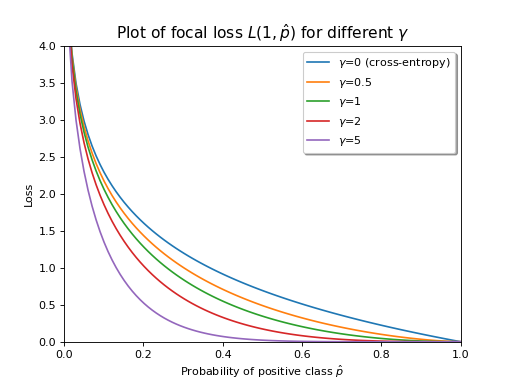
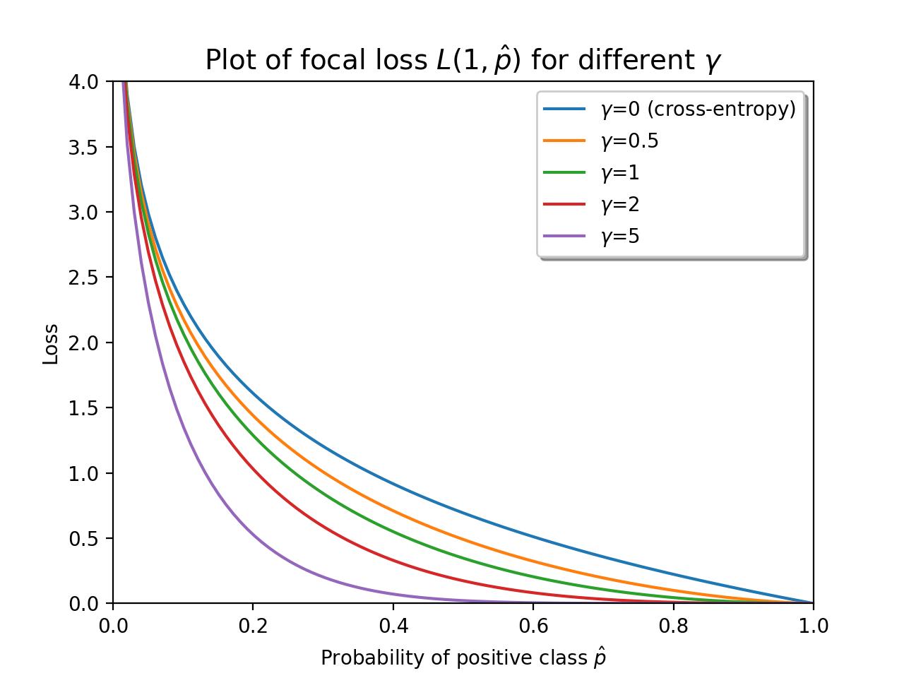
Below is a visualization of the focal loss between the positive class and predicted probabilities between 0 and 1. Note that as \(\gamma\) increases, the losses for predictions closer to 1 get smoothly pushed to 0.
import numpy as np
import matplotlib.pyplot as plt

from focal_loss import binary_focal_loss

ps = np.linspace(0, 1, 100)
gammas = (0, 0.5, 1, 2, 5)

plt.figure()
for gamma in gammas:
    loss = binary_focal_loss(1, ps, gamma=gamma)
    label = rf'$\gamma$={gamma}'
    if gamma == 0:
        label += ' (cross-entropy)'
    plt.plot(ps, loss, label=label)
plt.legend(loc='best', frameon=True, shadow=True)
plt.xlim(0, 1)
plt.ylim(0, 4)
plt.xlabel(r'Probability of positive class $\hat{p}$')
plt.ylabel('Loss')
plt.title(r'Plot of focal loss $L(1, \hat{p})$ for different $\gamma$',
          fontsize=14)
plt.show()
(Source code, png, hires.png, pdf)
Notes
A classifier often estimates the positive class probability \(\hat{p}\) by computing a real-valued logit \(\hat{y} \in \mathbb{R}\) and applying the sigmoid function \(\sigma : \mathbb{R} \to (0, 1)\) defined by
\[\sigma(t) = \frac{1}{1 + e^{-t}}, \qquad (t \in \mathbb{R}).\]That is, \(\hat{p} = \sigma(\hat{y})\). In this case, the focal loss can be written as a function of the logit \(\hat{y}\) instead of the predicted probability \(\hat{p}\):
\[L(y, \hat{y}) = -\alpha y \left(1 - \sigma(\hat{y})\right)^\gamma \log(\sigma(\hat{y})) - (1 - y) \sigma(\hat{y})^\gamma \log(1 - \sigma(\hat{y})).\]This is the formula that is computed when specifying from_logits=True. However, this formula is not very numerically stable if implemented directly; for example, there are multiple log and sigmoid computations involved. Instead, we use some tricks to rewrite it in the more numerically stable form
\[L(y, \hat{y}) = (1 - y) \hat{p}^\gamma \hat{y} + \left(\alpha y \hat{q}^\gamma + (1 - y) \hat{p}^\gamma\right) \left(\log(1 + e^{-|\hat{y}|}) + \max\{-\hat{y}, 0\}\right),\]where \(\hat{p} = \sigma(\hat{y})\) and \(\hat{q} = 1 - \hat{p}\) denote the estimates of the probabilities of the positive and negative classes, respectively.
Indeed, starting with the observations that
\[\log(\sigma(\hat{y})) = \log\left(\frac{1}{1 + e^{-\hat{y}}}\right) = -\log(1 + e^{-\hat{y}})\]and
\[\log(1 - \sigma(\hat{y})) = \log\left(\frac{e^{-\hat{y}}}{1 + e^{-\hat{y}}}\right) = -\hat{y} - \log(1 + e^{-\hat{y}}),\]we obtain
\[\begin{split}\begin{aligned} L(y, \hat{y}) &= -\alpha y \hat{q}^\gamma \log(\sigma(\hat{y})) - (1 - y) \hat{p}^\gamma \log(1 - \sigma(\hat{y})) \\ &= \alpha y \hat{q}^\gamma \log(1 + e^{-\hat{y}}) + (1 - y) \hat{p}^\gamma \left(\hat{y} + \log(1 + e^{-\hat{y}})\right)\\ &= (1 - y) \hat{p}^\gamma \hat{y} + \left(\alpha y \hat{q}^\gamma + (1 - y) \hat{p}^\gamma\right) \log(1 + e^{-\hat{y}}). \end{aligned}\end{split}\]Note that if \(\hat{y} < 0\), then the exponential term \(e^{-\hat{y}}\) could become very large. In this case, we can instead observe that
\[\begin{split}\begin{align*} \log(1 + e^{-\hat{y}}) &= \log(1 + e^{-\hat{y}}) + \hat{y} - \hat{y} \\ &= \log(1 + e^{-\hat{y}}) + \log(e^{\hat{y}}) - \hat{y} \\ &= \log(1 + e^{\hat{y}}) - \hat{y}. \end{align*}\end{split}\]Moreover, the \(\hat{y} < 0\) and \(\hat{y} \geq 0\) cases can be unified by writing
\[\log(1 + e^{-\hat{y}}) = \log(1 + e^{-|\hat{y}|}) + \max\{-\hat{y}, 0\}.\]Thus, we arrive at the numerically stable formula shown earlier.
References
[1] T. Lin, P. Goyal, R. Girshick, K. He and P. Dollár. Focal loss for dense object detection. IEEE Transactions on Pattern Analysis and Machine Intelligence, 2018. (DOI) (arXiv preprint) See also
BinaryFocalLoss()- A wrapper around this function that makes it a
tf.keras.losses.Loss.